# /// script
# requires-python = ">=3.11"
# dependencies = [
# "matplotlib>=3.9",
# "pandas",
# "numpy",
# "scipy",
# "statsmodels",
# ]
# ///
import datetime
import warnings
warnings.filterwarnings("ignore")
import matplotlib
matplotlib.use("Agg")
import matplotlib.pyplot as plt
import matplotlib.patches as mpatches
from matplotlib.colors import LinearSegmentedColormap, Normalize, TwoSlopeNorm
from matplotlib.cm import ScalarMappable
from matplotlib.gridspec import GridSpec
from matplotlib.lines import Line2D
import numpy as np
import pandas as pd
from scipy.stats import gaussian_kde, linregress
from statsmodels.nonparametric.smoothers_lowess import lowess
# ── Data ──────────────────────────────────────────────────────────────────────
df = pd.read_csv("kyoto-cherry-blossoms-with-temps-bot-09818f.csv")
df = df.dropna(subset=["year", "day_of_year"]).copy()
df["year"] = df["year"].astype(int)
df["day_of_year"] = df["day_of_year"].astype(float)
df_temp = df.dropna(subset=["mar_mean_temp_c"]).copy()
MEAN_DAY = df["day_of_year"].mean()
YEAR_MIN = int(df["year"].min())
YEAR_MAX = int(df["year"].max())
YEAR_SPAN = YEAR_MAX - YEAR_MIN
df["dev"] = df["day_of_year"] - MEAN_DAY
df_s = df.sort_values("year").reset_index(drop=True)
# ── LOESS smooth + CI band ────────────────────────────────────────────────────
loess_out = lowess(df_s["day_of_year"], df_s["year"], frac=0.12, it=3,
return_sorted=True)
loess_x = loess_out[:, 0]
loess_y = loess_out[:, 1]
# CI: rolling SE of LOESS residuals (±1 SE band)
resid = df_s["day_of_year"].values - loess_y
HALF_WIN = 15
roll_se = np.array([
resid[max(0, i-HALF_WIN): i+HALF_WIN+1].std(ddof=1) /
np.sqrt(len(resid[max(0, i-HALF_WIN): i+HALF_WIN+1]))
for i in range(len(resid))
])
# ── Palette ───────────────────────────────────────────────────────────────────
BG = "#faf8f3"
TEXT = "#1e1b2e"
MUTED = "#9a918a"
GRID_C = "#e4dbd0"
# early bloom (neg dev) → rose/warm; late bloom (pos dev) → blue/cool
CMAP_DIV = LinearSegmentedColormap.from_list(
"bloom", ["#c9184a", "#e8a0bf", "#bfa8b8", "#a8c5da", "#1a6a9a"], N=512)
CMAP_YEAR = LinearSegmentedColormap.from_list(
"yr", ["#e8a0bf", "#9b59b6", "#1e1b2e"], N=256)
LOESS_COLOR = "#c9184a" # bold sakura pink
dev_lim = np.percentile(np.abs(df["dev"]), 97)
dev_norm = TwoSlopeNorm(vcenter=0, vmin=-dev_lim, vmax=dev_lim)
yr_norm = Normalize(df_temp["year"].min(), df_temp["year"].max())
matplotlib.rcParams.update({
"font.family": "sans-serif",
"font.sans-serif": ["DejaVu Sans"],
"text.color": TEXT,
"axes.labelcolor": TEXT,
"xtick.color": MUTED,
"ytick.color": MUTED,
"xtick.labelsize": 9,
"ytick.labelsize": 9,
"axes.facecolor": BG,
"figure.facecolor": BG,
"axes.grid": False,
})
# ── Layout ────────────────────────────────────────────────────────────────────
fig = plt.figure(figsize=(18, 22), facecolor=BG, dpi=150)
gs = GridSpec(2, 2, figure=fig,
height_ratios=[2.5, 1.6],
width_ratios=[1.55, 1.0],
hspace=0.12, wspace=0.28,
left=0.07, right=0.96, top=0.91, bottom=0.05)
ax1 = fig.add_subplot(gs[0, :])
ax2 = fig.add_subplot(gs[1, 0])
ax3 = fig.add_subplot(gs[1, 1])
for ax in [ax1, ax2, ax3]:
ax.set_facecolor(BG)
for sp in ax.spines.values():
sp.set_visible(False)
YTICKS = [84, 91, 100, 110, 121]
YLABELS = ["25 бер.", "1 квіт.", "10 квіт.", "20 квіт.", "1 трав."]
# ══ PANEL 1 – Timeline ════════════════════════════════════════════════════════
# Historical period bands — subtle fill + label on vertical divider
periods = [
(812, 1350, "#fff4ee"),
(1350, 1850, "#eef4ff"),
(1850, 2026, "#fff0f5"),
]
period_labels = [
(812, 1350, "Середньовічне потепління"),
(1350, 1850, "Мала льодовикова епоха"),
(1850, 2026, "Антропогенне потепління"),
]
for x0, x1, col in periods:
ax1.axvspan(x0, x1, color=col, alpha=0.55, zorder=0)
for x0, x1, lbl in period_labels:
ax1.text((x0 + x1) / 2, 126.5, lbl,
fontsize=8, color=MUTED, ha="center", va="bottom",
style="italic")
if x0 > 812:
ax1.axvline(x0, color=MUTED, lw=0.6, ls="--", alpha=0.35, zorder=1)
# Historical mean line
ax1.axhline(MEAN_DAY, color=MUTED, lw=0.9, ls="--", alpha=0.5, zorder=1)
UA_MONTHS = {1:"січ.",2:"лют.",3:"бер.",4:"квіт.",
5:"трав.",6:"черв.",7:"лип.",8:"серп.",
9:"вер.",10:"жовт.",11:"лист.",12:"груд."}
mean_doy = int(round(MEAN_DAY))
mean_dt = datetime.date(2024, 1, 1) + datetime.timedelta(mean_doy - 1)
mean_label = f"{mean_dt.day} {UA_MONTHS[mean_dt.month]} — середнє за {YEAR_SPAN} р."
ax1.text(YEAR_MIN + 8, MEAN_DAY + 0.5, mean_label,
fontsize=8, color=MUTED, va="bottom")
ax1.fill_between(loess_x, loess_y - roll_se, loess_y + roll_se,
color=LOESS_COLOR, alpha=0.14, zorder=2)
# Scatter — colored by deviation
ax1.scatter(df_s["year"], df_s["day_of_year"],
c=df_s["dev"], cmap=CMAP_DIV, norm=dev_norm,
s=18, alpha=0.62, linewidths=0, zorder=3)
# LOESS line
ax1.plot(loess_x, loess_y,
color=LOESS_COLOR, lw=2.4, alpha=0.90, zorder=4, solid_capstyle="round")
# ── Annotation helper: curved arrow, no box ──────────────────────────────────
def annotate_curved(ax, yr, dy, xtext, ytext, text,
ha="left", va="center", color=TEXT, rad=0.25,
marker="o", ms=3.5, fontweight="normal", arrowstyle="-|>"):
"""Curved-arrow annotation without box background."""
ax.annotate(
text, xy=(yr, dy), xytext=(xtext, ytext),
fontsize=8, fontweight=fontweight, color=color, ha=ha, va=va, zorder=7,
arrowprops=dict(
arrowstyle=arrowstyle,
color=color,
lw=0.9,
mutation_scale=7,
connectionstyle=f"arc3,rad={rad}",
),
annotation_clip=False,
)
ax.plot(yr, dy, marker, ms=ms, color=color, alpha=0.9, zorder=8)
# ── Global records (computed from data) ───────────────────────────────────────
row_earliest = df.loc[df["day_of_year"].idxmin()]
yr_earliest = int(row_earliest["year"])
dy_earliest = row_earliest["day_of_year"]
dt_earliest = datetime.date(2024, 1, 1) + datetime.timedelta(int(dy_earliest) - 1)
row_latest = df.loc[df["day_of_year"].idxmax()]
yr_latest = int(row_latest["year"])
dy_latest = row_latest["day_of_year"]
dt_latest = datetime.date(2024, 1, 1) + datetime.timedelta(int(dy_latest) - 1)
annotate_curved(ax1, yr_earliest, dy_earliest,
yr_earliest - 160, dy_earliest - 2.5,
f"{yr_earliest} — найраніше ({dt_earliest.day} {UA_MONTHS[dt_earliest.month]})",
ha="left", color="#c9184a", rad=-0.25,
marker="*", ms=10, fontweight="bold", arrowstyle="-")
annotate_curved(ax1, yr_latest, dy_latest,
yr_latest, dy_latest - 2,
f"{yr_latest} — найпізніше ({dt_latest.day} {UA_MONTHS[dt_latest.month]})",
ha="right", va="top", color="#1a6a9a", rad=-0.25,
marker="*", ms=10, fontweight="bold", arrowstyle="-")
# ── Per-period: earliest & latest, text clipped to period x-range ─────────────
period_ranges = [
(812, 1350, "#a0522d"),
(1351, 1850, "#457b9d"),
(1851, 2026, "#6b2d8b"),
]
MARGIN = 40 # min gap from period edge in years
for p0, p1, pcol in period_ranges:
sub = df[(df["year"] >= p0) & (df["year"] <= p1)]
if sub.empty:
continue
# ── Earliest ──
row_min = sub.loc[sub["day_of_year"].idxmin()]
yr_min = int(row_min["year"])
dy_min = row_min["day_of_year"]
dt_min = datetime.date(2024,1,1) + datetime.timedelta(int(dy_min) - 1)
lbl_min = f"{yr_min} ({dt_min.day} {UA_MONTHS[dt_min.month]})"
# ── Latest ──
row_max = sub.loc[sub["day_of_year"].idxmax()]
yr_max = int(row_max["year"])
dy_max = row_max["day_of_year"]
dt_max = datetime.date(2024,1,1) + datetime.timedelta(int(dy_max) - 1)
lbl_max = f"{yr_max} ({dt_max.day} {UA_MONTHS[dt_max.month]})"
skip_min = yr_min == yr_earliest
skip_max = yr_max == yr_latest
# Text x: prefer to the right of point but clipped inside [p0+MARGIN, p1-MARGIN]
if not skip_min:
# place text below & to the right, clipped to period
xt_min = float(np.clip(yr_min + 30, p0 + MARGIN, p1 - MARGIN))
yt_min = dy_min - 4 # below on standard axis
ha_min = "left" if xt_min >= yr_min else "right"
rad_min = -0.25 if xt_min >= yr_min else 0.25
annotate_curved(ax1, yr_min, dy_min, xt_min, yt_min, lbl_min,
ha=ha_min, va="top", color=pcol, rad=rad_min)
if not skip_max:
# place text above & to the left, clipped to period
xt_max = float(np.clip(yr_max - 30, p0 + MARGIN, p1 - MARGIN))
yt_max = dy_max + 4 # above on standard axis
ha_max = "right" if xt_max <= yr_max else "left"
rad_max = 0.25 if xt_max <= yr_max else -0.25
annotate_curved(ax1, yr_max, dy_max, xt_max, yt_max, lbl_max,
ha=ha_max, va="bottom", color=pcol, rad=rad_max)
# ── Data description — bottom-left, below the legend ─────────────────────────
ax1.text(0.01, 0.98,
"Кожна точка — зафіксована дата\n"
"пікового цвітіння сакури у Кіото.\n"
f"Колір: відхилення від {YEAR_SPAN}-річного\n"
f"середнього ({mean_dt.day} {UA_MONTHS[mean_dt.month]}).",
transform=ax1.transAxes, ha="left", va="top",
fontsize=8.5, color=MUTED, linespacing=1.5)
ax1.set_xlim(YEAR_MIN - 4, YEAR_MAX + 4)
ax1.set_ylim(80, 128) # standard: early bloom at bottom
ax1.set_yticks(YTICKS)
ax1.set_yticklabels(YLABELS)
ax1.yaxis.grid(True, color=GRID_C, lw=0.6, zorder=0)
ax1.xaxis.grid(True, color=GRID_C, lw=0.6, zorder=0)
# Legend
leg_items = [
Line2D([0], [0], color=LOESS_COLOR, lw=2.4, label="LOESS (frac = 0.12)"),
mpatches.Patch(color=LOESS_COLOR, alpha=0.22, label="\u00b11 SE"),
]
ax1.legend(handles=leg_items, loc="lower left", frameon=False,
fontsize=9, bbox_to_anchor=(0.01, 0.03), borderpad=0.8)
# Deviation colorbar — centered at MEAN_DAY position on the y-axis
# Replace standard colorbar with scattered points for a softer, airy look
ax1_pos = ax1.get_position()
y_lim_bot, y_lim_top = ax1.get_ylim() # (80, 128) — вісь не інвертована
mean_frac = (MEAN_DAY - y_lim_bot) / (y_lim_top - y_lim_bot) # ≈ 0.5
cbar_h = ax1_pos.height * 0.30
cbar_y0 = ax1_pos.y0 + mean_frac * ax1_pos.height - cbar_h / 2
cax1 = fig.add_axes([ax1_pos.x1 + 0.007, cbar_y0, 0.012, cbar_h])
y_vals = np.linspace(-12, 12, 50)
cax1.scatter(np.zeros_like(y_vals), y_vals, c=y_vals, cmap=CMAP_DIV, norm=dev_norm,
s=10, alpha=0.7, edgecolors="none")
cax1.set_ylim(-14, 14)
cax1.set_xlim(-0.5, 1)
cax1.axis("off")
# Add text labels manually
cax1.text(0.3, -12, "−12 дн.\n(раніше)", fontsize=7.5, color=MUTED, ha="left", va="center")
cax1.text(0.3, 0, "середнє", fontsize=7.5, color=MUTED, ha="left", va="center")
cax1.text(0.3, 12, "+12 дн.\n(пізніше)", fontsize=7.5, color=MUTED, ha="left", va="center")
cax1.text(0, 15, "Відхил.", fontsize=7.5, color=MUTED, ha="center", va="bottom")
# ══ PANEL 2 – Floral Calendar Heatmap ════════════════════════════════════════
df_heat = df.dropna(subset=["day_of_year"]).copy()
df_heat["century"] = (df_heat["year"] - 1) // 100 + 1
min_century = int(df_heat["century"].min())
max_century = int(df_heat["century"].max())
centuries = np.arange(min_century, max_century + 1)
# Create bins: Century edges, Day edges (in steps of 2)
cent_edges = np.arange(min_century - 0.5, max_century + 1.5)
day_min_h = int(np.floor(df_heat["day_of_year"].min() / 2) * 2) - 2
day_max_h = int(np.ceil(df_heat["day_of_year"].max() / 2) * 2) + 4
day_edges = np.arange(day_min_h, day_max_h, 2)
heatmap_data = np.zeros((len(centuries), len(day_edges)-1))
for i, cent in enumerate(centuries):
days_c = df_heat[df_heat["century"] == cent]["day_of_year"]
if len(days_c) > 0:
counts, _ = np.histogram(days_c, bins=day_edges)
heatmap_data[i] = counts / len(days_c) * 100 # percentage of blooms
heatmap_data[heatmap_data == 0] = np.nan
cmap_heat = LinearSegmentedColormap.from_list("sakura_heat", ["#ffc2d1", "#ff8fab", "#fb6f92", "#c9184a"])
cmap_heat.set_bad(color="none")
X, Y = np.meshgrid(day_edges, cent_edges)
mesh = ax2.pcolormesh(X, Y, heatmap_data, cmap=cmap_heat, edgecolors="white", linewidths=0.6, zorder=3)
# Highlight modern era (21st century) with a subtle box
ax2.plot([day_edges[0], day_edges[-1], day_edges[-1], day_edges[0], day_edges[0]],
[max_century - 0.5, max_century - 0.5, max_century + 0.5, max_century + 0.5, max_century - 0.5],
color="#c9184a", lw=1.5, zorder=4)
ax2.set_xlim(day_edges[0], day_edges[-1])
ax2.set_ylim(max_century + 0.5, min_century - 0.5)
ax2.set_yticks(centuries)
ax2.set_yticklabels([f"{c} ст." for c in centuries], fontsize=8.5)
ax2.set_xticks(YTICKS)
ax2.set_xticklabels(YLABELS, fontsize=8.5)
ax2.set_xlabel("Дата цвітіння", fontsize=10, labelpad=6)
ax2.set_title("Квітковий календар: зсув масового цвітіння",
fontsize=11, fontweight="bold", pad=10, loc="left")
ax2.xaxis.grid(False)
ax2.yaxis.grid(False)
# Colorbar for Frequency
cb_heat = fig.colorbar(mesh, ax=ax2, orientation="vertical",
pad=0.03, fraction=0.045, aspect=20)
cb_heat.set_label("Частота (%)", fontsize=9, color=MUTED)
cb_heat.ax.tick_params(labelsize=8, labelcolor=MUTED, color=MUTED)
cb_heat.outline.set_visible(False)
# ══ PANEL 3 – Temperature Distributions (Raincloud) ═══════════════════════════
df_t = df.dropna(subset=["apr_mean_temp_c", "year"]).copy()
periods_t = [
("1881–1910", 1881, 1910, 8.0),
("1911–1940", 1911, 1940, 6.0),
("1941–1970", 1941, 1970, 4.0),
("1971–2000", 1971, 2000, 2.0),
(f"2001–{YEAR_MAX}", 2001, YEAR_MAX, 0.0),
]
# X axis is Temperature
temp_min_all = df_t["apr_mean_temp_c"].min()
temp_max_all = df_t["apr_mean_temp_c"].max()
x_kde_t = np.linspace(temp_min_all - 1.0, temp_max_all + 1.0, 500)
lbl_x_pos = temp_min_all - 1.2 # x-position for period labels
line_x_start = temp_min_all - 1.1 # start of connecting dotted line
rng_t = np.random.default_rng(42)
for lbl, y0, y1, y_base in periods_t:
data = df_t[(df_t["year"] >= y0) & (df_t["year"] <= y1)]["apr_mean_temp_c"].values
if len(data) < 5:
continue
n_pts = len(data)
mean_val = data.mean()
q1, median, q3 = np.percentile(data, [25, 50, 75])
# Use a consistent bold pink for all periods to remove the fading effect
col = "#c9184a"
# 1. Cloud (KDE)
kde = gaussian_kde(data, bw_method=0.35)
yk = kde(x_kde_t)
yk_scaled = yk / yk.max() * 1.1 # max height is 1.1 (leaves 0.9 units empty above)
ax3.fill_between(x_kde_t, y_base, y_base + yk_scaled, alpha=0.35, color=col, lw=0)
# Baseline
kde_mask = yk > (yk.max() * 0.01)
x_min, x_max = x_kde_t[kde_mask].min(), x_kde_t[kde_mask].max()
ax3.plot([x_min, x_max], [y_base, y_base], color=col, lw=1.5)
# Mean diamond on baseline
ax3.plot(mean_val, y_base, marker="D", color=col, ms=6, zorder=6)
# Text above mean
mean_txt = f"{mean_val:.1f}°C"
ax3.text(mean_val, y_base + 0.15, mean_txt, color="white", fontweight="bold",
fontsize=8.5, ha="center", va="bottom",
bbox=dict(facecolor=col, edgecolor="none", pad=1.5, boxstyle="round,pad=0.2"))
# 2. Gray IQR Box (Aligned with points)
ax3.fill_between([q1, q3], y_base - 0.35, y_base - 0.05, color="#d3d3d3", alpha=0.85, zorder=2)
# Median line in box
ax3.plot([median, median], [y_base - 0.35, y_base - 0.05], color="white", lw=2, zorder=3)
# 3. Rain (Jittered dots, placed on the same level as the box)
jitter = rng_t.uniform(-0.35, -0.05, size=len(data))
ax3.scatter(data, y_base + jitter, color=col, s=12, alpha=0.7, edgecolors="white", linewidths=0.5, zorder=4)
# 4. Period label (Left side)
ax3.text(lbl_x_pos, y_base, lbl, color=col, fontsize=9.5, fontweight="bold", va="center", ha="right")
# Dotted line from text to cloud
if x_min > line_x_start:
ax3.plot([line_x_start, x_min], [y_base, y_base], color=col, ls=":", lw=1.5, alpha=0.7)
# 5. n points (Right side)
ax3.text(x_max + 0.2, y_base, f"n={n_pts}", color=col, fontsize=8, fontweight="bold", va="center", ha="left")
ax3.set_xlabel("Середня температура квітня (°C)", fontsize=10, labelpad=6)
ax3.set_title("Температурний дощ: потепління по 30-річчях",
fontsize=11, fontweight="bold", pad=10, loc="left")
ax3.set_xlim(lbl_x_pos - 2.3, temp_max_all + 2.0)
ax3.set_ylim(-1.0, periods_t[0][3] + 1.8)
ax3.xaxis.grid(True, color=GRID_C, lw=0.5)
ax3.yaxis.set_visible(False)
ax3.spines["left"].set_visible(False)
ax3.spines["top"].set_visible(False)
ax3.spines["right"].set_visible(False)
# ── Global title & footer ──────────────────────────────────────────────────────
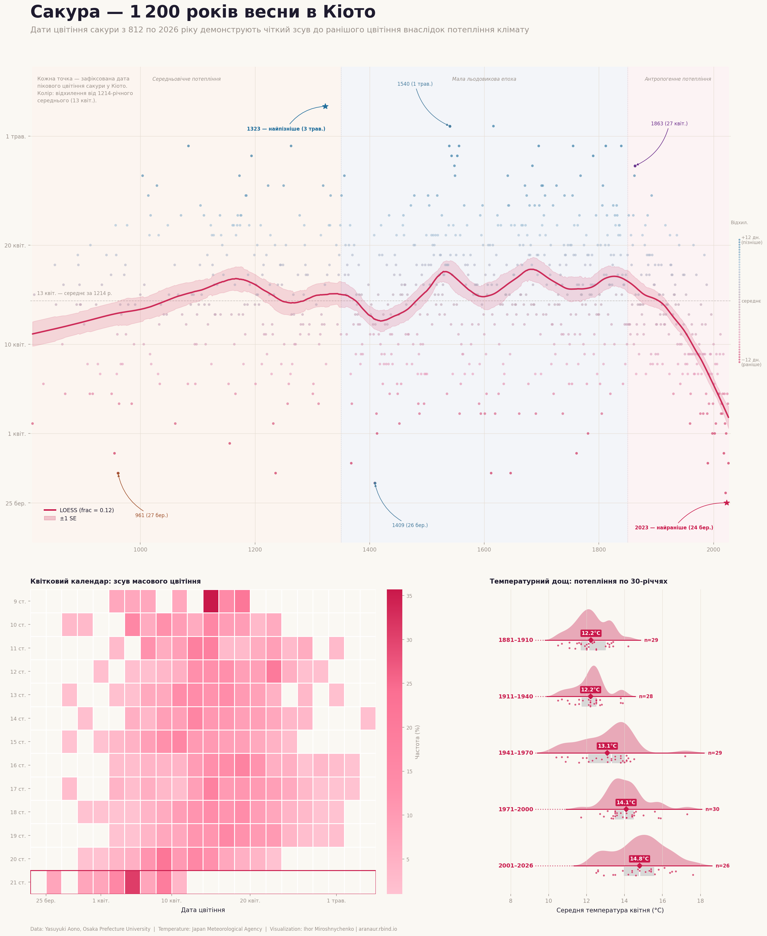
fig.text(0.07, 0.975, "Сакура \u2014 1\u2009200 років "
"весни в Кіото",
fontsize=28, fontweight="bold", color=TEXT, va="top")
fig.text(0.07, 0.952,
"Дати цвітіння сакури з 812 по 2026 року "
"демонструють чіткий зсув до ранішого "
"цвітіння внаслідок потепління клімату",
fontsize=13, color=MUTED, va="top")
fig.text(0.07, 0.012,
"Data: Yasuyuki Aono, Osaka Prefecture University | "
"Temperature: Japan Meteorological Agency | Visualization: Ihor Miroshnychenko | aranaur.rbind.io",
fontsize=8, color=MUTED, ha="left")
# ── Save ──────────────────────────────────────────────────────────────────────
plt.savefig("sakura_plot.png", dpi=150, bbox_inches="tight", facecolor=BG)
print("Saved: sakura_plot.png")